2025-12-11 13:58:08

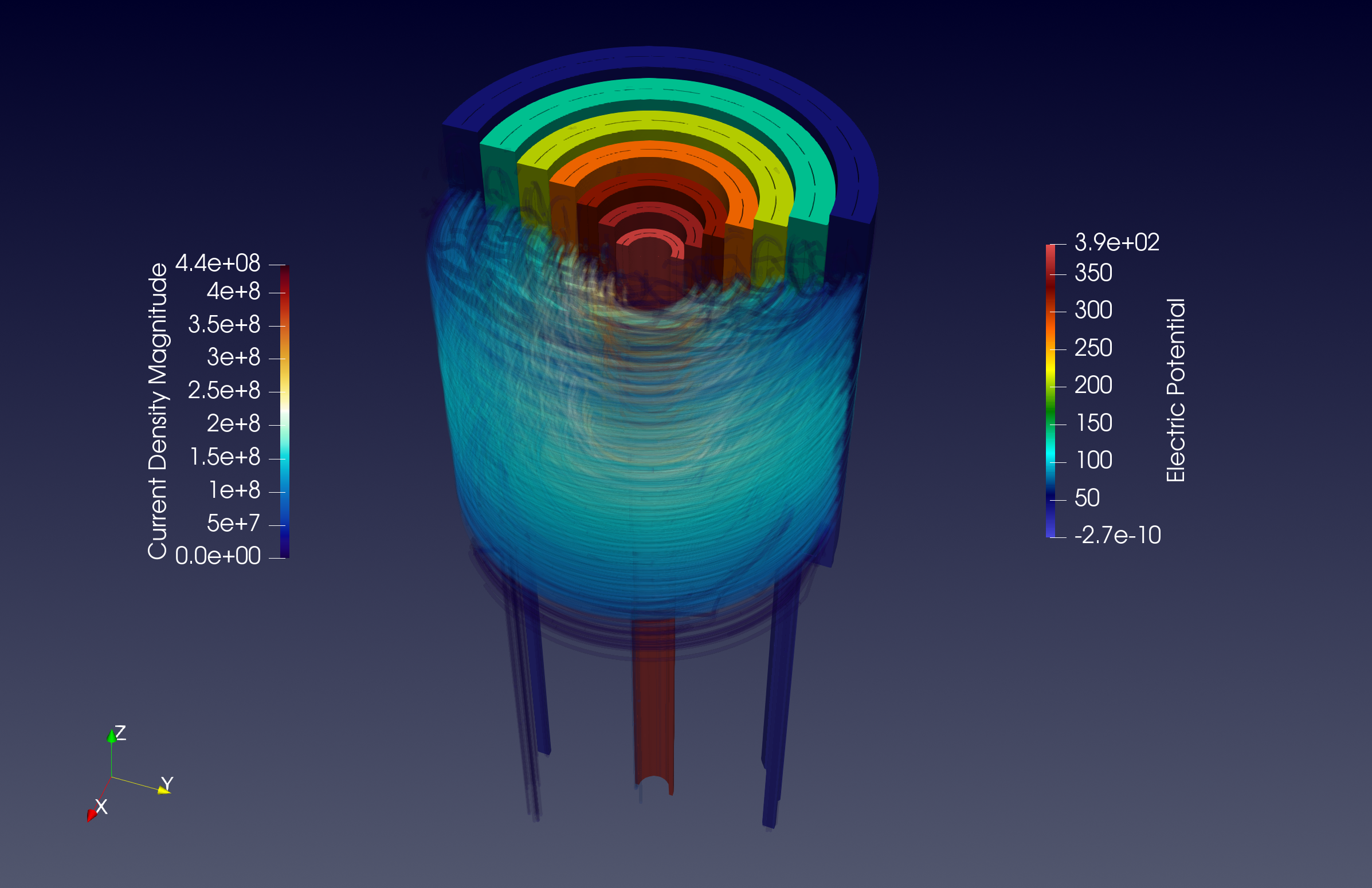
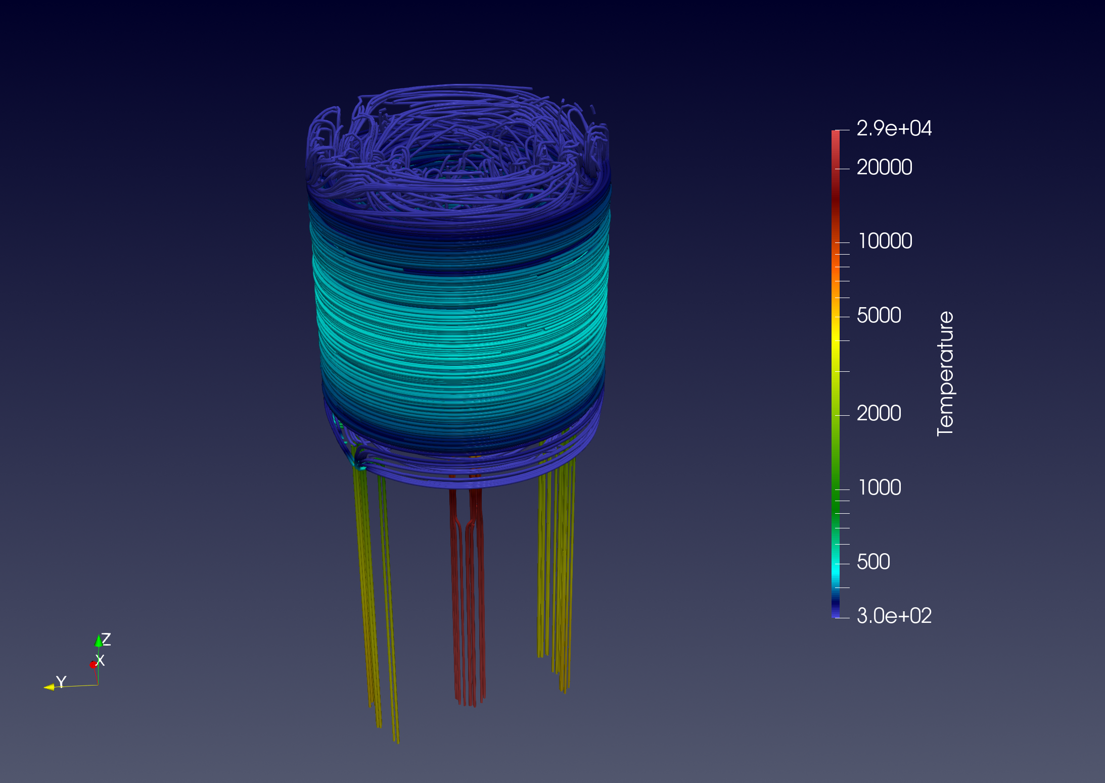
This benchmark models the temperature field and electric current distribution in an high field resistive magnet of the Laboratoire National des Champs Magnétiques Intenses. The magnet consist in a set of 14 copper alloys cylindrical tubes connected 2 by 2 into series by rings. In each tube, the current path is defined by 2 helical cuts of 0.2 mm width. The rings are machined to let water flow in between each tube in a channel of 0.8 mm. The magnet is operated at 12 MW with an imosed total current of 31 kA. The water flow in the magnet is about 140 l/s. The water cooling of the magnet is modelling by using Robin boundary conditions with parameters derived from classical correlation in thermo-hydraulics. A more detailled version of the full model is available in (Daversin Catty, 2016; Hild, 2020). The model is run with thermoelectric Feel++ toolbox. The geometry used in this benchmark performance is illustrated in Figure 4.13. This is a complex domain composed of a large number of components, with some very thin parts.

This benchmark was done using feelpp.benchmarking, version 4.0.0

The benchmark was performed on the gaya supercomputer (see Section 10.1). The performance tools integrated into the Feel-toolboxes framework were used to measure the execution time. Moreover, we need to say that we have used several Feel installations.

Note: the Feel++ version is identical but the dependencies (like Petsc) which are of course more recent with Noble.

The metrics measured are the execution time of the main components of the simulation. We enumerate these parts in the following:

We can find in fig. 4.14 some examples of 3D visualization that represent fields obtained by solving the thermoelectric problem. We have the temperature solution and other quantities evaluated at PostProcess phase such as current density, electric potential, and electric fields.

The performance analysis has been done in two supercomputers, Gaya and Discoverer. For each of them, we have run the benchmark with discretizations P1 and P2. About the Feel++ distribution, we use native Ubuntu Jammy packages for Gaya, and Apptainer (with Ubuntu) for Discoverer. The results on these machines are illustrated in figs. 4.15 and 4.16 respectively. The measures presented are the time-consuming of simulation components related to WP1, namely Init, Assembly, and PostProcess. For the Solve component, we refer to section 6.2.3.3.

In each case analyzed, we have very good scalability, in the sense that we reduced significantly the execution time by increasing the number of tasks. The Init phase is the most timeconsuming, with a limit quite high compared to others. This part contains the mesh reading from the disk, which can explain some bumps sometimes when require many HPC resources.

To conclude, we can say that we successfully ran this benchmark case, and we are ready to go up to larger problems and more complex modeling.

HPC experiments with other kinds of discretizations

Go to extreme HPC scale: Partitioning and IO issues